Image Captioning Project

Exploring the dataset

This project builds on the Microsoft Common Objects in COntext (MS COCO) dataset The dataset is commonly used to train and benchmark object detection, segmentation, and captioning algorithms.

You can read more about the dataset on the website or in the research paper.

Step 1: Initialize the COCO API

We begin by initializing the COCO API that you will use to obtain the data. This project builds on the train2014 dataset. It’s provides sufficient data for our model to generalize. Later, the model is evaluated on the val2014 and test2014 dataset.

Step 2: Plot a Sample Image

Next, we plot a random image from the dataset, along with its five corresponding captions. Each time you run the code cell below, a different image is selected.

In the project, you will use this dataset to train your own model to generate captions from images!

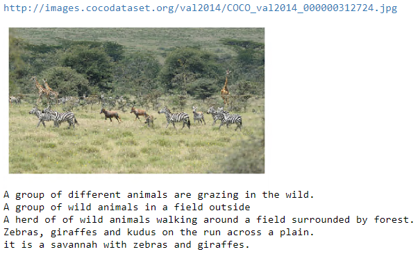
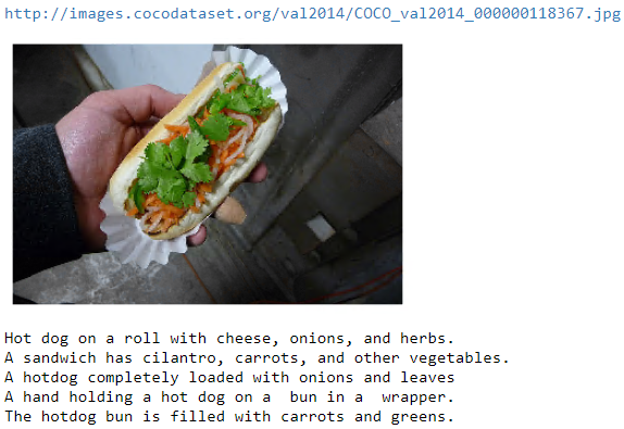
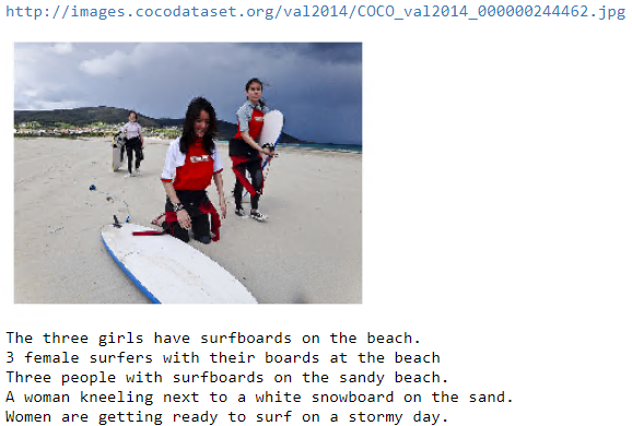
Above are three examples of training data in our dataset. As we can see, each image is pared with 5 captioning written by different people. The captionings are not necessarily of the same length and they have different focuses of the image.

Out Objective is to devise a neural network that takes an image an input, and generate a caption that reasonably describe the input image.

The architecture of our model is described as below:

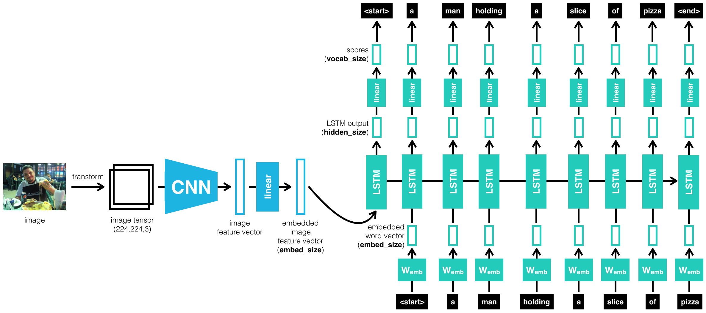
We have a CNN-RNNencoder-decoder architecture where the CNN encodes the image into a feature_vector of a fixed size (embed_size). The decoder (RNN) receives the feature_vector and generates a sequence of words that described the content in the input image.

The above image demonstrate the end-to-end training process of the model where the image feed to the model and it’s output are compared with the ground-truth captioning to compute loss. Details of the architecture are discussed in model.py file.

Step 3: Explanations of details in data_loader and model.py

We use data loader to load the COCO dataset in batches.

In the code cell below, you will initialize the data loader by using the get_loader function in data_loader.py.

The data_loader.py is in a separate file that contains all these detail.

The get_loader function takes as input a number of arguments that can be explored in data_loader.py. Take the time to explore these arguments now by opening data_loader.py in a new window. Most of the arguments must be left at their default values, and you are only allowed to amend the values of the arguments below:

1. transform - an image transform specifying how to pre-process the images and convert them to PyTorch tensors before using them as input to the CNN encoder. We can choose our own image transform to pre-process the COCO images.
2. mode - one of 'train' (loads the training data in batches) or 'test' (for the test data). We will say that the data loader is in training or test mode, respectively. While following the instructions in this notebook, please keep the data loader in training mode by setting mode='train'.
3. batch_size - determines the batch size. When training the model, this is number of image-caption pairs used to amend the model weights in each training step. Typically, we start with a batch_size of 32 and increase or decrease empirically.
4. vocab_threshold - the total number of times that a word must appear in the in the training captions before it is used as part of the vocabulary. Words that have fewer than vocab_threshold occurrences in the training captions are considered unknown words.
5. vocab_from_file - a Boolean that decides whether to load the vocabulary from file.

We will describe the vocab_threshold and vocab_from_file arguments in more detail soon.

Once we have specified the above variables, we can create our data_loader from COCO training dataset. NOTE THAT: the vocab_threshold parameters we have specified will influence vocabulary we obtain from the dataset. Basically, we will label all words that have appear less than vocab_threshold as

Exploring the __getitem__ Method

The data loader was stored in the variable data_loader.

We can access the corresponding dataset as data_loader.dataset. This dataset is an instance of the CoCoDataset class in data_loader.py. If you are unfamiliar with data loaders and datasets, you are encouraged to review this PyTorch tutorial.

The __getitem__ method in the CoCoDataset class determines how an image-caption pair is pre-processed before being incorporated into a batch. This is true for all Dataset classes in PyTorch; if this is unfamiliar to you, please review the tutorial linked above.

When the data loader is in training mode, this method begins by first obtaining the filename (path) of a training image and its corresponding caption (caption).

Image Pre-Processing

Image pre-processing is relatively straightforward (from the __getitem__ method in the CoCoDataset class):

# Convert image to tensor and pre-process using transform
image = Image.open(os.path.join(self.img_folder, path)).convert('RGB')
image = self.transform(image)

After loading the image in the training folder with name path, the image is pre-processed using the same transform (transform_train) that was supplied when instantiating the data loader.

Caption Pre-Processing

The captions also need to be pre-processed and prepped for training. In this example, for generating captions, we are aiming to create a model that predicts the next token of a sentence from previous tokens, so we turn the caption associated with any image into a list of tokenized words, before casting it to a PyTorch tensor that we can use to train the network.

To understand in more detail how COCO captions are pre-processed, we’ll first need to take a look at the vocab instance variable of the CoCoDataset class. The code snippet below is pulled from the __init__ method of the CoCoDataset class:

def __init__(self, transform, mode, batch_size, vocab_threshold, vocab_file, start_word, 
        end_word, unk_word, annotations_file, vocab_from_file, img_folder):
        ...
        self.vocab = Vocabulary(vocab_threshold, vocab_file, start_word,
            end_word, unk_word, annotations_file, vocab_from_file)
        ...

From the code snippet above, you can see that data_loader.dataset.vocab is an instance of the Vocabulary class from vocabulary.py. Take the time now to verify this for yourself by looking at the full code in data_loader.py.

We use this instance to pre-process the COCO captions (from the __getitem__ method in the CoCoDataset class):

# Convert caption to tensor of word ids.
tokens = nltk.tokenize.word_tokenize(str(caption).lower())   # line 1
caption = []                                                 # line 2
caption.append(self.vocab(self.vocab.start_word))            # line 3
caption.extend([self.vocab(token) for token in tokens])      # line 4
caption.append(self.vocab(self.vocab.end_word))              # line 5
caption = torch.Tensor(caption).long()                       # line 6

Every caption is added a special start word: <start> and a special end word: <end>. So a sentence like: ‘A person doing a trick on a rail while riding a skateboard’ will be tokenized as: [0, 3, 98, 754, 3, 396, 39, 3, 1009, 207, 139, 3, 753, 18, 1] where 0 stands for <start> and 1 stands for <end>.

During prediction, when we receive a <end> from the model, it would also mean we terminate producing captioning.

Finally, this list is converted to a PyTorch tensor. All of the captions in the COCO dataset are pre-processed using this same procedure from lines 1-6 described above.

As you saw, in order to convert a token to its corresponding integer, we call data_loader.dataset.vocab as a function. The details of how this call works can be explored in the __call__ method in the Vocabulary class in vocabulary.py.

def __call__(self, word):
    if not word in self.word2idx:
        return self.word2idx[self.unk_word]
    return self.word2idx[word]

The word2idx instance variable is a Python dictionary that is indexed by string-valued keys (mostly tokens obtained from training captions). For each key, the corresponding value is the integer that the token is mapped to in the pre-processing step.

Batching in the Data_Loader

The captions in the dataset vary greatly in length. We can examining using data_loader.dataset.caption_lengths. The majority of them are around 10, and there are captions that go up to 50+ length.

To generate batches of training data, we begin by first sampling a caption length (where the probability that any length is drawn is proportional to the number of captions with that length in the dataset). Then, we retrieve a batch of size batch_size of image-caption pairs, where all captions have the sampled length. This approach for assembling batches matches the procedure in this paper and has been shown to be computationally efficient without degrading performance.

Run the code cell below to generate a batch. The get_train_indices method in the CoCoDataset class first samples a caption length, and then samples batch_size indices corresponding to training data points with captions of that length. These indices are stored below in indices.

These indices are supplied to the data loader, which then is used to retrieve the corresponding data points. The pre-processed images and captions in the batch are stored in images and captions.

Model architecture

EncoderCNN

For Encoder we used the ResNet50 model pre-trained from image-nets. More powerful model can be applied here. However, ResNet50 performs reasonably well with a decent amount of training. We would freeze all the weights in the pre-trained model and remove its output layer. The removed output layer is replaced with our own Linear layer that takes in the number of output features and produce a feature of size: embedding size. Therefore, it is important that when creating an instance of our EncoderCNN model we make sure to take in parameter embed_size to specify our network sufficiently.

The Encoder takes in an image of (224,224,3) and produce an feature vector of (embed_size).

DecoderRNN

The decoder is a simple LSTM architecture with dropout for regularization. When specifying out decoder, make sure we have the correct vocab_size which is determined when we decide our vocab_threshold and construct our Vocabulary. It is also important to imbed our target captions using nn.Embedding() first before feeding into our network.

Notice that we have input length of (1+len(captions)), the “1” comes from our image feature vector. Therefore, for the hidden state of LSTM we only take hiddens[:,:-1,:] so that the lengths match. The structure is demonstrated below:

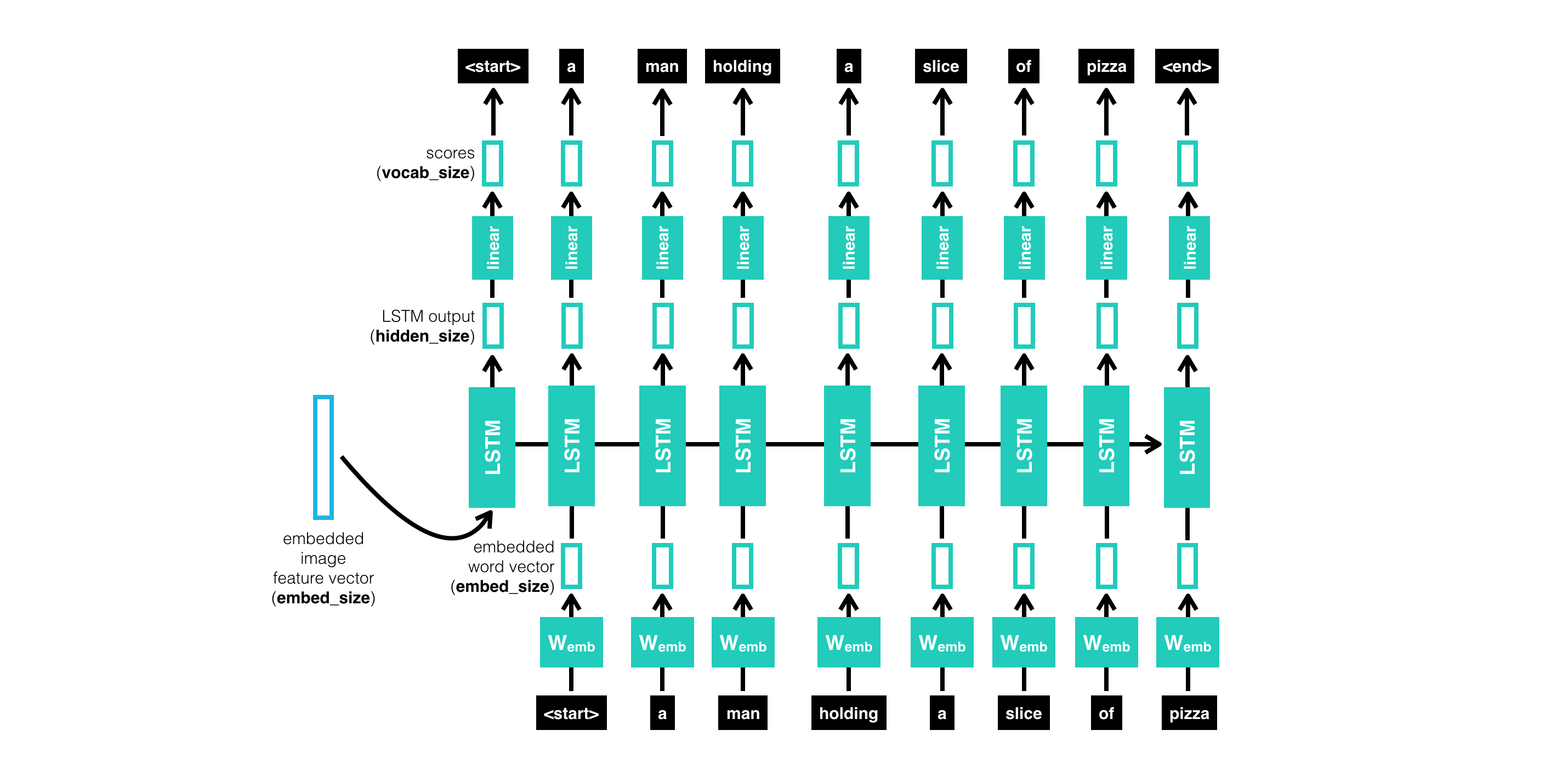
Things we need to decide when creating instances of our network: embed_size from the input image, hidden_size for the DecoderRNN, vocab_size from the vocabulary we created earlier and the number of layers for our LSTM.

Training

Now, we start training in the Training.ipynb file.

Important parameters that effects the training of our network:

• batch_size - the batch size of each training batch. It is the number of image-caption pairs used to amend the model weights in each training step.
• vocab_threshold - the minimum word count threshold. Note that a larger threshold will result in a smaller vocabulary, whereas a smaller threshold will include rarer words and result in a larger vocabulary.
• vocab_from_file - a Boolean that decides whether to load the vocabulary from file.
• embed_size - the dimensionality of the image and word embeddings.
• hidden_size - the number of features in the hidden state of the RNN decoder.
• num_epochs - the number of epochs to train the model. We recommend that you set num_epochs=3, but feel free to increase or decrease this number as you wish. This paper trained a captioning model on a single state-of-the-art GPU for 3 days, but you’ll soon see that you can get reasonable results in a matter of a few hours! (But of course, if you want your model to compete with current research, you will have to train for much longer.)
• save_every - determines how often to save the model weights. We recommend that you set save_every=1, to save the model weights after each epoch. This way, after the ith epoch, the encoder and decoder weights will be saved in the models/ folder as encoder-i.pkl and decoder-i.pkl, respectively.
• print_every - determines how often to print the batch loss to the Jupyter notebook while training. Note that you will not observe a monotonic decrease in the loss function while training - this is perfectly fine and completely expected! You are encouraged to keep this at its default value of 100 to avoid clogging the notebook, but feel free to change it.
• log_file - the name of the text file containing - for every step - how the loss and perplexity evolved during training.

We applied nn.CrossEntropuLoss() in this case to compute our loss. Adam optimizer are used for optimization with learning rate of 0.0001. The neural network is trained for 3 Epochs. The loss is initialized to be 9.3 and drops to around 2. There is a lot of potential of improving the training such as using adaptive learning rate, applying a different optimizer or simply spend more time in training.

Inference

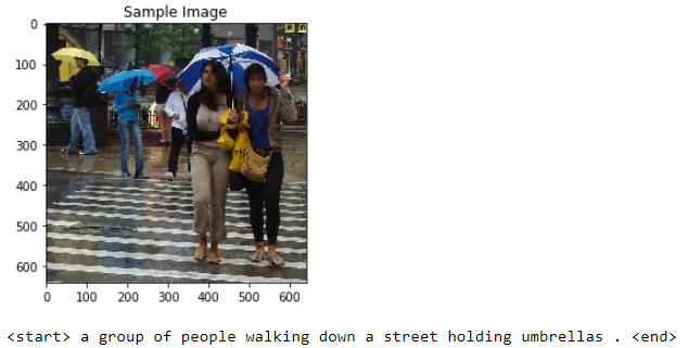
Finally, let test our trained model by feeding the encoder an unseen image from test dataset and ask our decoder to perform captioning based on the encoded feature vector.

The maximum of caption is 25 words and we end prediction we the word <end> is computed at any given time step.

More Evaluation

This is the most basic model we can come up with to do image-captioning. The model is a quite simple, but it has the right architecture to produce reasonable description.

Next up

we will see cases where the model performed well and cases where our model failed. From the failures, we shall summaries the type of mistakes our model make and propose potential remedies.

The model performed well:

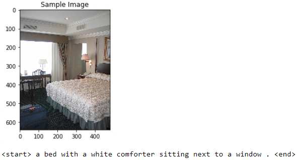
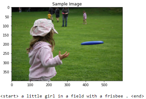
In these two examples, the model does recognize the objects in the images and captured the main idea of what is going on.

Now, let’s see cases where model could have performed better …

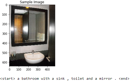
Remark: There is sink and mirror, but there is no toilet! What is potentially happening here is that: in our training images, toilet usually appear together with sinks and mirrors. So our DecoderRNN has learnt to assiciate “bathroom pixel features” with all of those since they often come up together in the training captions. This is not surprising to see, in that we build a “seq-to-seq” model where our DecoderRNN only gets one input(encoded image feature). In the following time-steps, our decoder only depend on predicted words from previous output(prediction from last time-step). Thus, if the word toilet appeared together with sink and mirror in training dataset, the words are likely to come up together in predictions.

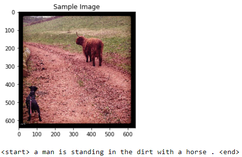
Remark: There is neither man nor horse in the picture but a dog and a cattle. Definitely wrong species!

We could argue that the figure of the dog reasonably resembles a human figure and the cattle is not very different from a horse(surely more furry). This mistake might have to do with how the model has learnt to associate the objects in the image with the backgrounds. It could be the likelihood of human and horse appearing in dirt and grass is bigger than that of a dog and a cattle.

How can we do better?

Dwelling on the mistakes we usually make, besides the limited training tuning we have done, I would say that it has a lot to do with how we constructed our model. More specifically, our Decoder gets the image encoder as the input at the first time-step. Afterwards, all predictions depend on the predicted word in the last time-step.

This is not very ideal for two main reasons:

1. Decoder only gets to see the input image at first time-step. It would be a lot more intuitive if the encoder gets to make each word prediction while referring back to different part of the image. (This would avoid “seeing” a dog and say it’s a human, I expect) In addition, if each word’s prediction could associate back to some part of the image, we should expect less decency among words themselves.
2. The sequence of words that our model predicts has a lot to do with our first word selection. Namely, if the model were to choose a terrible first word, it would be unlikely that it perform great captioning afterwards.

To remedy these problems, we are going to implement more sophisticated model with Attention Mechanism, and Beam Search during decoding in order to boost our performance.

The implementations of the model are shown in my other GitHub repo.

See you there