Sequence_Labeling_Project

Linguistic sequence labeling is a general approach encompassing a verity of problems. One of the crucial reason that this repo exists is because a collection of techniques used in this project is one of the building blocks of my surgical robotics vision project. In addition to that, we are going to replicate the architecture used in the Empower Sequence Labeling with Task-Aware Neural Language Model paper, which is considered as one of the more sophisticated models out there for tasks such as Poart-Of-Speech (POS) and Named-Entity-Recognition (NER). This paper is packed of useful techniques that can be potentially extended to other deep learning applications.

Acknowledgement, this repo is heavy guided by sgrvinod‘s tutorial and also a few ideas that I have learned from the FastAI course v3.

NER

Overview

Architecture

The development of deep neural networks made it possible for us to build reliable models for POS and NER tasks without handcrafting features. The paper provides us with a very concise and robust model and incorporates both word-level information as well as character-level information. In addition, the architecture also features transfer learning the knowledge from another related task. However, this is not done in the traditional transfer learning way but realized by conducting multi-task learning. (the details of multi-task training strategy will be covered in the next section)

LM_LSTM_CRF

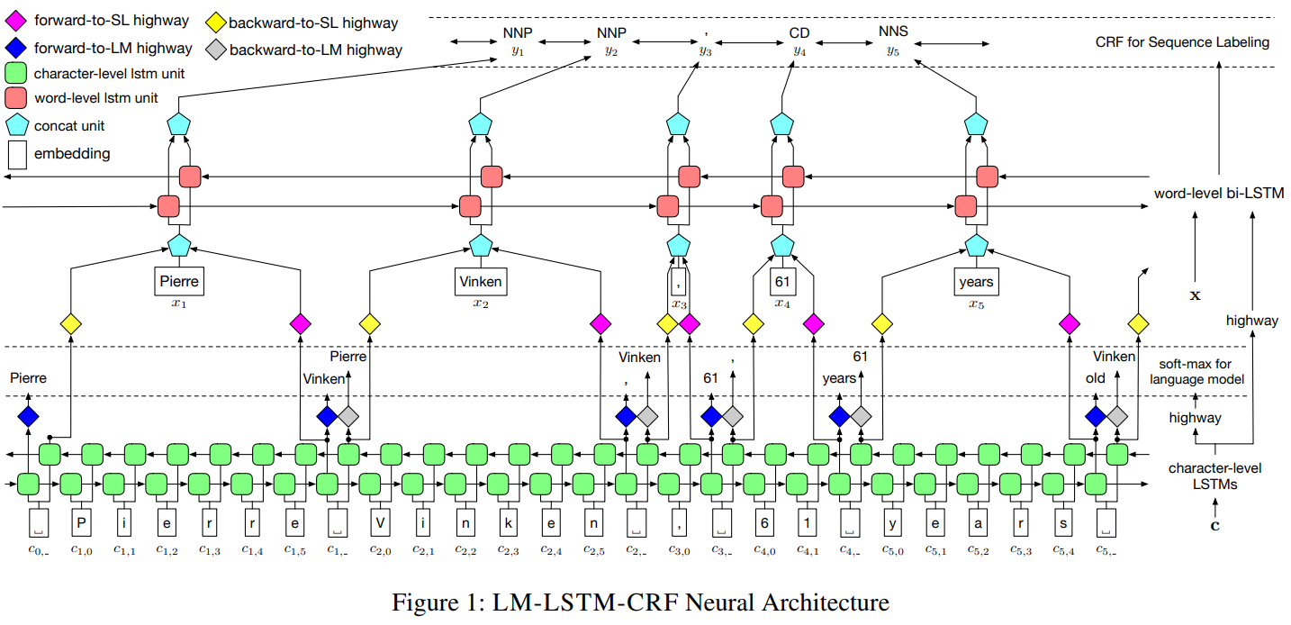
The model is called LM-LSTM-CRF which is essentially the concatenation of the important techniques they have applied. The model, which is very well described as above, looks fairly complicated at first glance. A lot of things seem to be going on at the same time. Don’t worry, I will decouple them for you later and you will realize that the great result that this architecture achieved comes from a smart combination of a few useful deep learning tricks.

As the name suggests, the model has three main components:

Character-level LSTMs(there are two of them, one forward one backward) that is trained concurrently with a language model.
Word-level bi-directional LSTM with additional input of high-way connections from features extracted by character-level LSTM
Conditional Random Field as the output layer that eventually performs the labelling

Character-level LSTMs

The objective of this layer come in two folds:

Chracter-level feature extractions that will be used as parts of input for word-level LSTM
Neural language model training(this multi-task training strategy is used to boost model’s performance)

There are two character-level LSTMs that extracts feature by reading the documents in, forward direction and backward direction, respectively.

As shown below, the output of these two LSTMs(in blues) are flowing to two places:

predicting next word(this is the language model part)
concatenated together to be used as part of input for word-level bidirectional LSTM

LM_LSTM

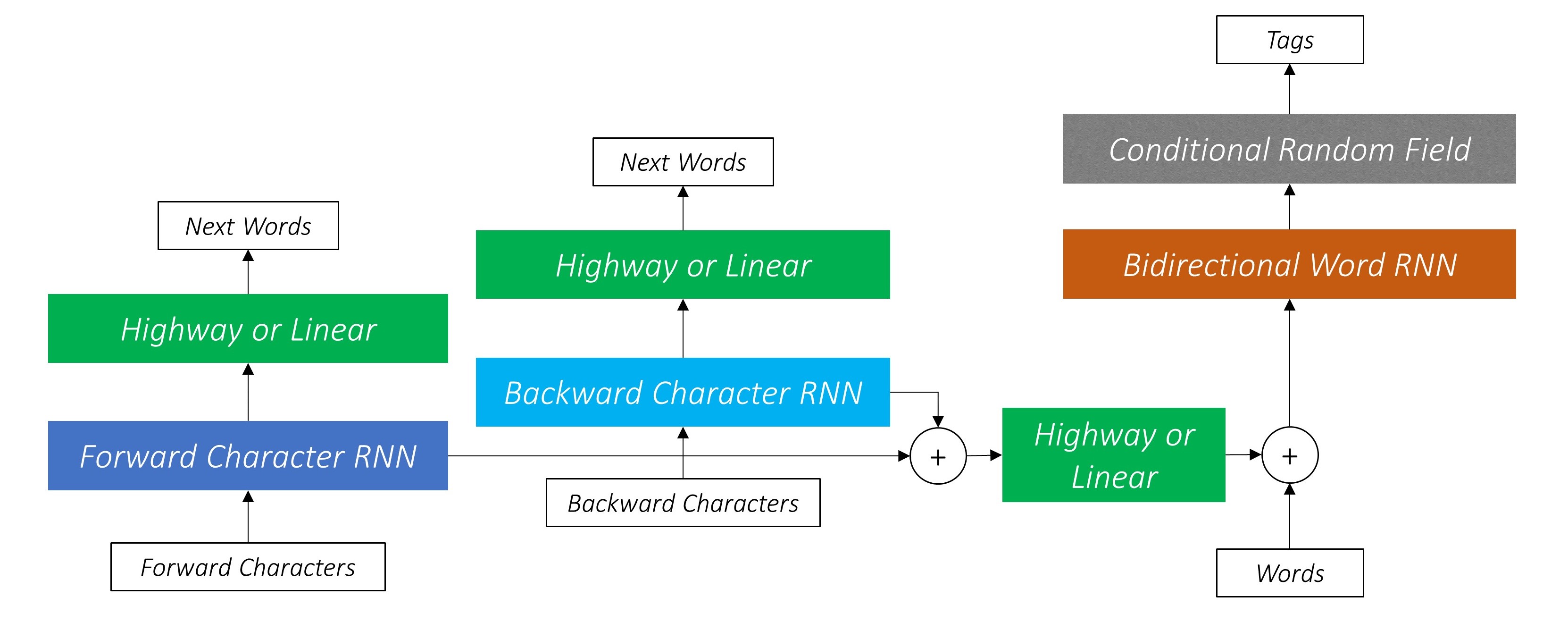
Note that the outputs of character-level has the option of passing through **Highway connections **(this concept will be explained in the technique section). For now, we can think of them as linear connections with more advance computations.

Finally, there is one more thing we need to decide when designing the architecture: when performing back-propagation, how is the error going to be aggregated from the two source(namely, one from predicting next word another from the main tasks itself). In the paper, the authors take weighting of $1:1$. Since this repo is an exact replica, we will take it. For the more advanced weighting strategy please refer to this paper where we can devise the loss with two learnable parameters that learns to balance the loss ratio.

Word-level Bi-directional LSTM

The Bi-directional LSTM take input of a concatenation of word sequence(after passing through pre-trained word embeddings) and features extracted by character-level LSTM. We are able to directly use bi-lstm here since we are not doing multi-task training, hence we can satisfied with getting the combined features of bi-lstm.

CRF for sequence labeling

CRF stands for conditional random fields which is popularly used to model ordered information. The output of bi-lstm is passed through CRF before the actually labeling is made. Taking a step back, a more naive approach is to take the activation from the bi-lstm and just sample the most possible tag for that given activation. First of all, this is not a bad strategy at all. However, CRF could potentially do better because it allows us to leverage more information when making the decision.

Put in simple words, instead of merely consider the give activation, CRF allows the model to compute the possibility of the sampling each tag GIVEN the neighborhood tags. The math behind is that, instead of only compute the emission scores (from bi-lstm activations), we also compute the transition score which represent the likelihood of sampling the tag i given the previous word was assigned to tag j.

Last word for architecture

So there you have it, this more advanced model architecture. It’s super sophisticated and effective but not so difficult to understand after all.

In a nutshell, we have 3 streams of information being fed into the word-level bi-lstm: the feature extraction from forward character-level lstm, the feature extraction from backward character-level lstm, and the word-level information itself.

# character-level
cf, _ = self.forw_char_lstm(cf)  
cb, _ = self.back_char_lstm(cb)   

# Unpack packed sequence
cf, _ = pad_packed_sequence(cf, batch_first=True)
cb, _ = pad_packed_sequence(cb, batch_first=True) 

# gather character-level info to the right word-level position
cf_selected = torch.gather(cf, 1, index=cmarkers_f) 
cb_selected = torch.gather(cb, 1, index=cmarkers_b)

# concate forward and backward; pass through high-way connection
subword = self.subword_hw(self.dropout(torch.cat((cf_selected, cb_selected), dim=2)))
subword = self.dropout(subword)

# Embedding look-up for words
w = self.word_embeds(wmaps) 
w = self.dropout(w)

# Concatenate word embeddings and sub-word features
w = torch.cat((w, subword), dim=2) # ready for bi-lstm

Techniques

What makes this paper special is the collection of useful techniques the authors choose to apply to the architecture in order to boost the performance. We are going to focus on a few, namely, multi-task learning, neural language model, viterbi decoding and high-way connections.

Multi-task Learning

A technique that has revolutionized the computer vision world (and potentially the NLP world as well by ULMFiT) is transfer learning. Essentially, researchers have learned that we can transfer the knowledge we have learned from different but related task if some basic rules are met. Multi-task learning is similar to transfer learning in a way that when we have limited training data, we can boost the performance of our model by the leveraging the knowledge learned from another task. Only this time, the training of different tasks happens concurrently. The character-level lstm model is trained along side a neural language model. Which essentially means that the output of the character-level lstm will be used in the two different tasks and there will be two loss gradients flowing back during the back-prop stage.

It was worth noting that, the implementation isn’t as simple as “let’s plug everything in together”. It was found by the authors that, based on experiments, when the tasks are discrepant, language model trainings could be harmful to sequence labeling in a naive co-training setting. This is understandable because without proper regulation, we have no necessary grantee that by training the character-level lstm to be better language models is always going to beneficial to the sequence labeling task. To mitigate this challenge, the authors proposed to apply high-way connections in order to transform the output of character-level lstm into different semantic space. With this understanding in mind, now it’s good time to introduce neural language model and high-way connections.

Neural language model

This is a family of models that are often used for article generation(#Shakespeare). Actually, not just word generation, they works on any types of sequence generation. The neural language modeling problem can be mathematically formulated as follows:

$p_f(x_1,\...,x_n)=\prod_{i=1}^{N}p_f(x_i|x_1,\...,x_{i-1})$

Which translates to English as: give a sequence of words, what is the likelihood the next word for all words in the vocabulary.

In the implementation of this sequence labeling project, two neural language models are training concurrently with the forward and backward character level lstm with the objective of improving model accuracy. As the authors pointed out: However, different from typical models of this setting, our two tasks are not strongly related. This discordance makes our problem more challenging.

To mediate these two tasks, the authors transform the output of character-level layers into different semantic spaces for different objectives. This strategy allows character-level layers to focus on general feature extraction and lets the transform layers select task-specific features. Hence, the language model can provide related knowledge to the sequence labeling, without forcing it to share the whole feature space.

Highway Networks

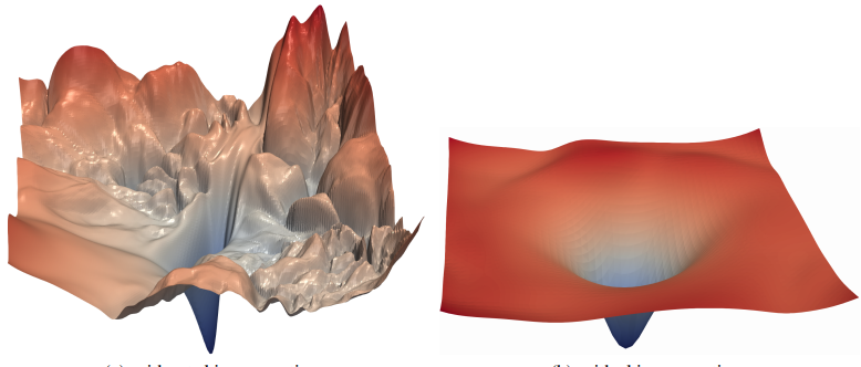
There is a famous CNN architecture in computer vision call ResNet in which there are many residual blocks. What researchers found is that the incorporation of residual blocks allow us to train much deeper networks with good convergence. When researchers try to visualize the loss surfaces of CNN with(right) and without(left) residual blocks, they found that the existence of residual connections greatly smoothen out the loss surface and made it more possible for the optimizer to find the global minimum.

Loss_surfaces

This could also be explained from another perspective by looking the residual connection formula:

$output=conv\_block(x)+x$

Therefore, the conv_block could decide to learn nothing and produce a value of 0 , thus the whole block will give a result same as its input essentially ‘bypass’ the whole unit. This flexibility eventually allow gradient to flow smoothly through much deeper net. Note that in this formulation, we can actually replace the conv_block() by any general transformation function:

$output=f(x)+x$

Building upon that, high-way connection is basically one more additional element away. We will be adding a gating to the structure so that there will be a sigmoid-activated gate(recall that sigmoid return a value between 0 and 1) deciding the weighting between original input and transformed value. Hence we have a connection that will return the input itself if the input is close negative infinity and the transformed activation if the input is close to positive infinity. 50/50 if input x is close to 0.

$output=g(x)f(x)+(1-g(x))x$

Viterbi decoding

During inference time, since we are not naively predicting labels based on emission scores, we need a way to generate a sequence of label based on the CRF matrix. Viterbi decoding helps us do just that. It considers not the likelihood of a certain tag based on the emission score itself as well as the previous tag and next tags. The best sequence of tags are selected based on the cumulative scores taken from the CRF matrix.

Realization

The code is realized with PyTorch in this file in the repo.

Since it’s a replica of the original implementation of the paper, we are going to test on the same benchmark dataset: the CoNLL 2003 NER dataset (Tjong Kim Sang and De Meulder 2003).

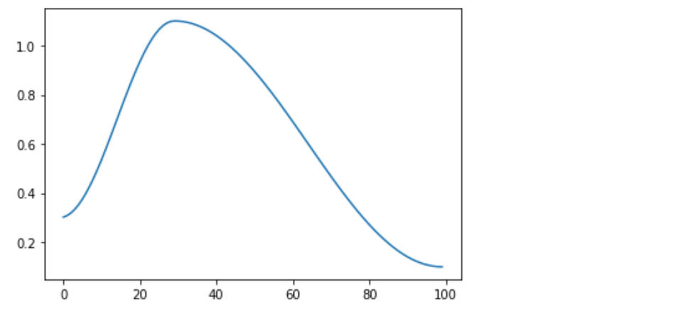
The only minor modification we will be making is to the learning_rate. Instead of gradually decaying the leraning_rate based on the current epochs, we will apply learning rate annealing technique. More specifically, a cosine annealing as shown below:

cosine_annealing

Highway connection

To realize the following computation, we will create a Hightway module that has a flexible number of layers:

$output=g(x)f(x)+(1-g(x))x$

class Highway(nn.Module):
    """
    Highway network
    """
    def __init__(self, size, num_layers=1, dropout=0.5):
        """
        size: size of Linear layer (should match input size)
        num_layers: number of transform and gate layers
        dropout: dropout rate
        """
        super(Highway, self).__init__()
        self.size = size
        self.num_layers = num_layers
        self.transform = nn.ModuleList() # A list of transform layers
        self.gate = nn.ModuleList()      # A list of gate layers
        self.dropout = torch.nn.Dropout(p=dropout)

        for i in range(num_layers):
            transform = nn.Linear(size, size)
            gate = nn.Linear(size, size)
            self.transform.append(transform)
            self.gate.append(gate)
    def forward(self, x):
        """
        Forward-prop.
        Returns a tensor with the same dimensions as input tensor
        """

        transformed = F.relu(self.transform[0](x))  # transform with the first transform layer
        g = F.sigmoid(self.gate[0](x))              # calculate how much of the transformed input to keep
        out = self.dropout(g*transformed + (1-g)*x)               # combine input and transformed input with ratio of g

        # If there are additional layers
        for i in range(self.num_layers):
            transformed = F.relu(self.transform[i](out))
            g = F.sigmoid(self.gate[i](out))
            out = self.dropout(g*transformed+(1-g)*out)

        return out

In our implementation, we will keep the num_layers as 1 layer. This will be applied in three different places in our architecture.

Conditional Random Fields

The math behind is that, instead of only compute the emission scores (from bi-lstm activations), we also compute the transition score which represent the likelihood of sampling the tag i given the previous word was assigned to tag j.

class CRF(nn.Module):
    """
    Confitional Random Field
    """

    def __init__(self, hidden_dim, tagset_size):
        """
        hidden_dim: the size of word/BLSTM's output (which is the input size for CRF)
        tagset_size: number of tags(depending on our dataset)
        """

        super(CRF, self).__init__()
        self.tagset_size = tagset_size
        self.emission = nn.Linear(hidden_dim, self.tagset_size)
        self.transition = nn.Parameter(torch.Tensor(self.tagset_size, self.tagset_size))
        self.transition.data.zero_() # initializa the transition matrix to be all zeros

    def forward(self, feats):
        """
        feats:   output of word/BLSTM, a tensor of dimensions-(batch_size, timesteps, hidden_dim)
        returns: CRF scores, a tensor of dimensions-(batch_size, timesteps, tagset_size, tagset_size)
        """
        self.batch_size = feats.size(0)
        self.timesteps  = feats.size(1)

        emission_scores = self.emission(feats)  # (batch_size, timesteps, tagset_size)
        # here we broadcast emission_scores in order to compute the total score later with transition score
        emission_scores = emission_scores.unsqueeze(2).expand(self.batch_size, self.timesteps, self.tagset_size, self.tagset_size)  # (batch_size, timesteps, tagset_size, tagset_size)

        crf_scores = emission_scores + self.transition.unsqueeze(0).unsqueeze(0)  # (batch_size, timesteps, tagset_size, tagset_size)
        return crf_scores

Connected after word-bidirectional-lstm to compute scores for word tags.

Viterbi-Loss

This is the loss to be used together with CrossEntropyLoss() for back-prop:

class ViterbiLoss(nn.Module):
    """
    Viterbi Loss.
    """

    def __init__(self, tag_map):
        """
        :param tag_map: tag map
        """
        super(ViterbiLoss, self).__init__()
        self.tagset_size = len(tag_map)
        self.start_tag = tag_map['<start>']
        self.end_tag = tag_map['<end>']

    def forward(self, scores, targets, lengths):
        """
        Forward propagation.
        :param scores: CRF scores
        :param targets: true tags indices in unrolled CRF scores
        :param lengths: word sequence lengths
        :return: viterbi loss
        """

        batch_size = scores.size(0)
        word_pad_len = scores.size(1)

        # Gold score

        targets = targets.unsqueeze(2)
        scores_at_targets = torch.gather(scores.view(batch_size, word_pad_len, -1), 2, targets).squeeze(
            2)  # (batch_size, word_pad_len)

        # Everything is already sorted by lengths
        scores_at_targets = pack_padded_sequence(scores_at_targets, lengths, batch_first=True)
        gold_score = scores_at_targets.data.sum()

        # All paths' scores

        # Create a tensor to hold accumulated sequence scores at each current tag
        scores_upto_t = torch.zeros(batch_size, self.tagset_size).to(device)

        for t in range(max(lengths)):
            batch_size_t = sum([l > t for l in lengths])  # effective batch size (sans pads) at this timestep
            if t == 0:
                scores_upto_t[:batch_size_t] = scores[:batch_size_t, t, self.start_tag, :]  # (batch_size, tagset_size)
            else:
                # We add scores at current timestep to scores accumulated up to previous timestep, and log-sum-exp
                # Remember, the cur_tag of the previous timestep is the prev_tag of this timestep
                # So, broadcast prev. timestep's cur_tag scores along cur. timestep's cur_tag dimension
                scores_upto_t[:batch_size_t] = log_sum_exp(
                    scores[:batch_size_t, t, :, :] + scores_upto_t[:batch_size_t].unsqueeze(2),
                    dim=1)  # (batch_size, tagset_size)

        # We only need the final accumulated scores at the <end> tag
        all_paths_scores = scores_upto_t[:, self.end_tag].sum()

        viterbi_loss = all_paths_scores - gold_score
        viterbi_loss = viterbi_loss / batch_size

        return viterbi_loss

Surgical_robotics_vision

This part will be completed when I start uploading my Surgical robotics vision project.