ULMFiT practical projects

In this repo, we will be reading and understanding two papers in details: the Universal Language Model Fine_tuning for Text Classification paper and the AWD-LSTM paper . Comparing ULMFiT to other models that are popularly applied in similar tasks such as language modeling and sentiment classification.

You will find three parts of contents in this repo:

• a deep dive into ULMFiT paper and the AWD-LSTM paper(the base architecture of ULMFiT)
• practical application of ULMFiT on IMDB sentiment classification
• what if we are interested in modeling a language that is not English?

Acknowledgement: Sincere thanks to Jeremy Howard, Sebastian Ruder and Rachel Thomas not just because that they wrote the ULMFiT paper, but more amazingly, for having developed the FastAI NLP course that provides users with interactive tutorials of implementation and practical advices.

Overview of critical techniques from papers

ULMFiT

ULMFiT stands for “Universal Language Model Fine-tuning for Text Classification”.

Motivation

It is widely know that in the field of computer vision, transfer learning has made a huge impact in both the model performance and the required training time to obtain robust models. On the other hand, existing approaches in NLP field, prior to this paper, has largely rely on task-specific modifications and training from scratch. In addition to that, it was not because that transfer learning was an unknown technique to the NLP specialists, but rather they consider NLP as a special field where domain knowledge is too task-specific to be built upon any general knowledge training until Jeremy and Sebastian have proven otherwise.

Contribution

ULMFiT shines to be the first paper that applies transfer learning in the field of NLP. In addition, Jeremy et al. introduce techniques that are crucial for fine-tuning such a language model.

“LMs overfit to small datasets and suffered catastrophic forgetting when fine-tuned with a classifier.” This was what’s hindering the development of applying transfer learning in NLP prior to ULMFiT. In short, if we bluntly training the entire layers with target task domain data, most of the useful information transfered from source task will be lost, hence denoted as ineffective. This problem was nicely addressed with the ULMFiT fine-tuning strategy which we will be getting into details later.

Model architecture and training strategy

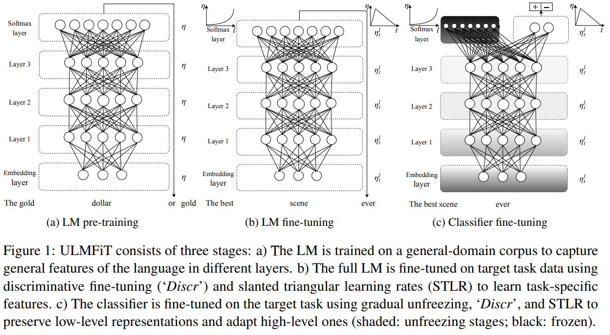
The base architecture, which is fully responsible for language modeling, is AWD-LSTM. Haven’t heard of it? Dont worry, we will be getting into the details of AWD-LSTM paper in the next section. For now, all we need to know is that it is the state-of-the-art language model in 2017 which builds upon a regular LSTM(with no attention, short-cut connections, or other sophisticated additions) with various tuned dropout hyper-parameters.

P.S: We can also use a transformer in the place of AWD-LSTM or basically any high performance language model. However, in this repo, we will be focusing on AWD-LSTM since it’s used in the original paper.

• Training step 1: General-domain LM pretrianing

Similar to what happens in CV transfer learning. Here we will be training our language model(AWD-LSTM) on a large corpus of general knowledge text. (Wiki-103 dataset is used)

• Training step 2: Target task LM fine-tuning

Fine-tuning the language model on the target task domain. Techniques such as: discriminative fine-tuning, slanted triangular learning rates are used. (we will be getting into the details later)

• Training step 3: Target task classifier fine-tuning

Classifier layers are added to the model structure, and we start to training the model on the actual task.

Important fine-tuning techniques

As mentioned before, ULMFiT has incorporated several powerful fine-tuning techniques that made the robust inductive transfer learning all possible.

Discriminative fine-tuning. As different layers capture different types of information, they should be fine-tuned to different extent(at different learning rate). In this implementation, the learning rate of the current layer is simply $\frac{1}{2.6}$ of the last layer.(with the top layer have highest learning rate).

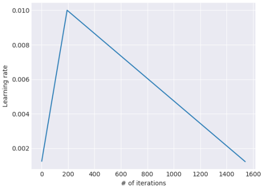
Slanted triangular learning rates. This is an specific implementation of learning rate scheduling, in that we apply different learning rates at different stages of the training. The one used in ULMFiT looks like this:

Gradual unfreezing. Rather than fine-tuning all layers at once, which risks catastrophic forgetting. Jeremy et al. found that by gradually unfreezing the layers from top-to-bottom greatly mitigate this issue. This was because the top layer contains the least general knowledge, and we should fine-tune the most sensitive layers(bottom layers) last when top layers are relatively stable.

Bidirectional language model. Training a forward LM that read in the default direction and training a backward LM that read backwards. Then combine the decision made by the two model in some manner(could be simply taking the average). This technique is likely to further improve the model accuracy.

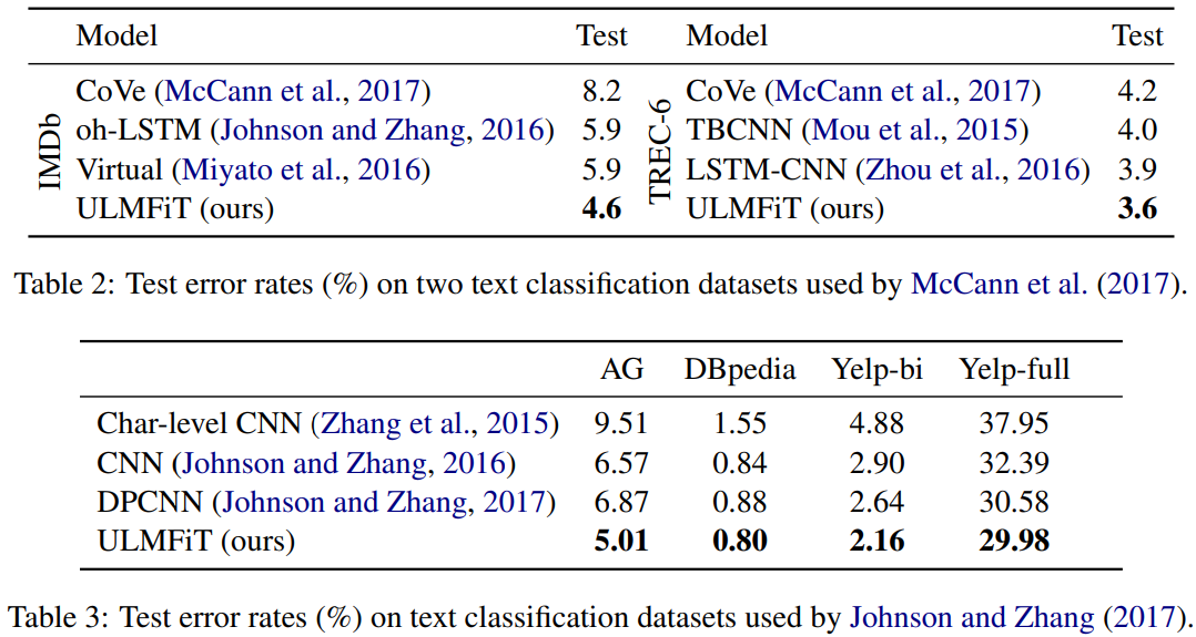
Performance comparison with similar models

AWD-LSTM paper

Recurrent neural networks serves as a fundamental building block for many sequence learning tasks before the transformer came along. The ULMFiT method adopts one high performance variation that features weight-dropped Long short-term memory (LSTM). In addition, a novel optimizer (NT-ASGD) was proposed to be applied in the training strategy.

Weight-dropped LSTM

LSTM can be formulated as:

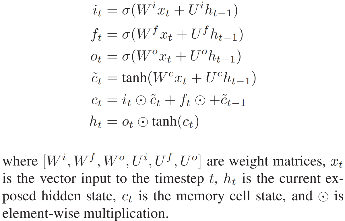
DropConnect was implemented in the architecture in that weight matrices are dropped before the forward and backward pass.

Variational dropout. In standard dropout, a new binary dropout mask is sampled each and every time the dropout function is called. Variational dropout only samples a dropout mask upon the first call and then will repeatedly use that locked dropout mask for all repeated connections within the forward and backward pass.

The values used for dropout on the word vectors, the output between LSTM layers, the output of the final LSTM layer, and embedding dropout were (0.4, 0.3, 0.4, 0.1), respectively.

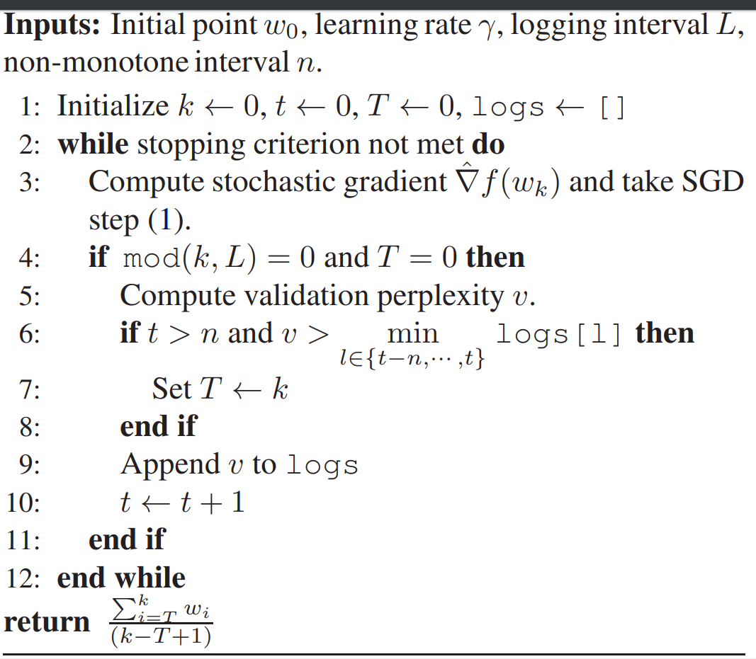
Non-monotonically Triggered ASGD(NT-ASGD)

This a variation of averaged Stochastic Gradient Descend which goes as follows:

ULMFiT Basics and implementation in sentiment analysis

If you are familiar with the techniques FastAI endorses when implementing transfer learning, the pipeline should look very familiar to you.(If not, check out my other repo) In order to build a deep learning model that classifies IMDb reviews, we only need 4 step:

1. Loading IMDb data and exploratory data analysis(EDA)
2. Formatting the data in a way that is ready for your DL framework of choice(in this case FastAI)
3. Fine-tuning the language model (from general wiki-text to domain specific)
4. Building a classifier on top of the fine-tuned language model

Contrary to Image transfer learning, texts can’t be directly transformed into numbers and be fed into our model. We need to conduct a two-step process, firstly tokenized the texts as a list of words(usually a vocabulary is associated) and secondly pass the tokenized words through an embedding layer to numericalize them

Mixed Precision Training

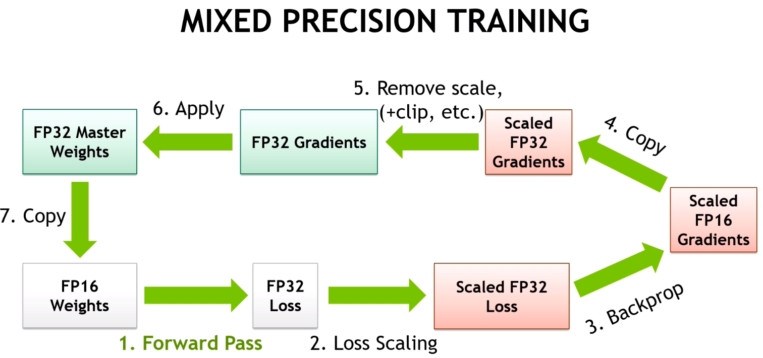
The motivation is to reduced both the amount of computation made in the network as well as storage required at the cost of using less precise data (fp16 is essentially half-precision as compared to fp 32). As a result, we will have faster training and potentially better performance.

• It turns our that sometimes, making things less precise in deep learning causes it to generalize a bit better.

  												-*Jeremy Howard*
  

The details about mixed precision training can be found in NVIDIA’s documentation. Simply put, NVIDIA has done a great job to optimize the GPU training process by converting part of the computation into half-precision-points such as back-prop’s gradients, activations in the forward pass.

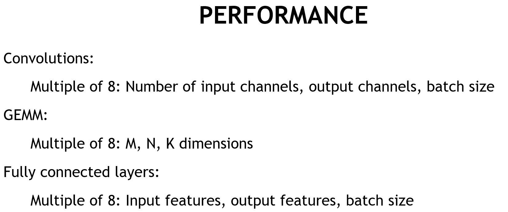
The following is the recommended model architecture recommended by NVIDIA for best GPU effciency:

Implementation of ULMFiT with FastAI

Step I: construct our dataset

In fastai we use the notion of databunch which is essentially PyTorch dataset paired with a dataloader with its corresponding transformations.

# we will use the IMDb dataset from FastAI repo
path = untar_data(URLs.IMDB) # this give us the directory to construct labeled text list

bs = 48
data_lm = (TextList.from_folder(path)                        # other options are also available such as `from_csv`
          .filter_by_folder(includ=['train','test','unsup']) # exclude other folders
          .split_by_rand_pct(0.1, seed=48)					 # randomly split 10-90
          .label_for_lm()									 # label as to predict the next word token
          .databunch(bs=bs))								 # convert to databunch for the learner later

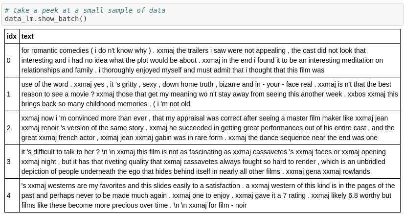
# Now if we call `show_batch()`
data_lm.show_batch()

This give us the following show batch:

Step II: create a Learner

The Learner concept in FastAI is an object that contains the databunch we just created as well as the model architecture and the optimizer we are going to use later. The amazing part is this could be done in just one line:

# the drop_mult decide the percentage of dropout to use in relation to the combination used in the original paper
learn_lm = language_model_learner(data_lm, AWD_LSTM, drop_mult=0.3)

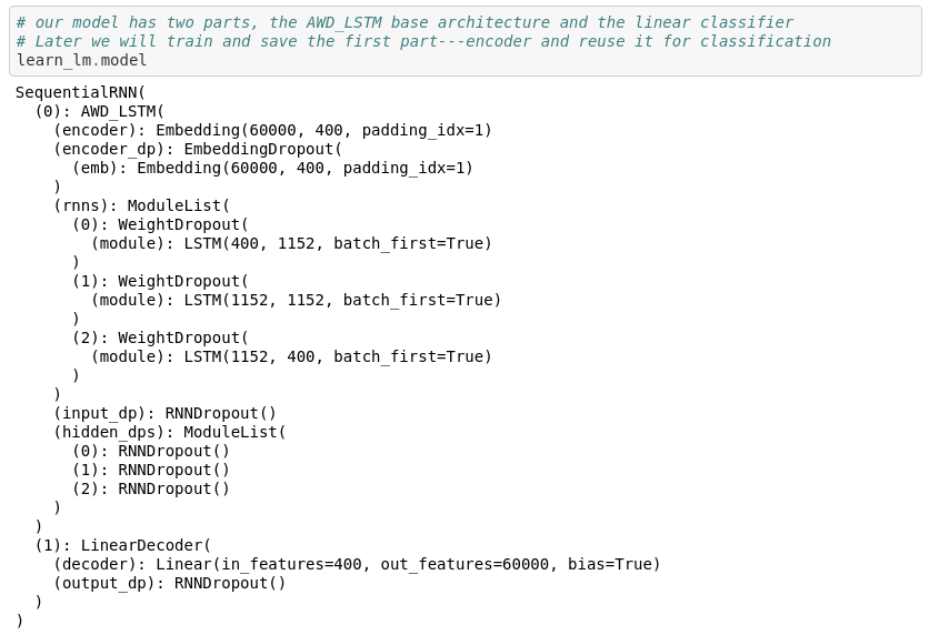
In this notebook, we will be using the same base architecture as the original paper: AWD_LSTM. We will be sure to explore more advanced base architectures with ULMFiT approach in my later posts, so don’t miss out. Now let’s take a good at this simple 3 layer structure:

Step III: training the language model

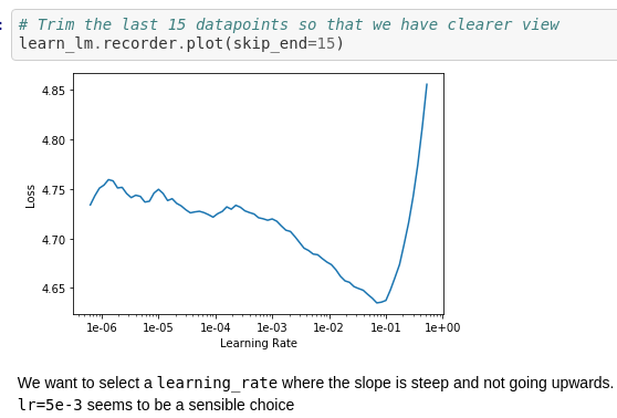
In FastAI we have a neat function to help us finding a sensible learning_rate. (isn’t this fantastic?)

learn_lm.lr_find()
# Trim the last 15 datapoints so that we have clearer view
learn_lm.recorder.plot(skip_end=15)

Then train the model with learn_lm.freeze() and train again with learn_lm.unfreeze():

# We want to select a learning_rate where the slope is steep and not going upwards.
# seems to be a sensible choice

lr=5e-3
learn_lm.to_fp16()
learn_lm.fit_one_cycle(5, lr, moms=(0.8,0.7))

# unfreeze and train again
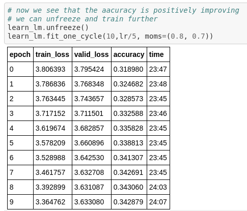
learn_lm.unfreeze()
learn_lm.fit_one_cycle(10,lr/5, moms=(0.8, 0.7))

The accuracy reflect how well the learner could get the absolute correct next word give previous words:

Step IV: Create the classification model

Now our language model is more IMDB like. We will proceed to train the classifier which is actually what we are about. Again, we will be creating a Databunch object , where this time, we are .split_by_folder() and .label_from_folder() :

bs = 48
data_clas = (TextList.from_folder(path, vocab=data_lm.vocab)
             #grab all the text files in path
             .split_by_folder(valid='test')
             #split by train and valid folder (that only keeps 'train' and 'test' so no need to filter)
             .label_from_folder(classes=['neg', 'pos'])
             #label them all with their folders
             .databunch(bs=bs, num_workers=1))

Of course, we will not be training from scratch this time. So the obvious thing to do here is to load the previously trained encoder when creating our Learner object:

learn_clas = text_classifier_learner(data_clas, AWD_LSTM, drop_mult=0.3)
learn_clas.load_encoder('fine_tuned_lm_enc')
learn_clas.freeze()

Step V: final training

The training process is similar to that of language model previously. In addition, we will be performing gradual unfreezing during fine-tuning our classifier.

Fine-tuning the target classifier is the most critical part of the transfer learning method. Overly aggressive fine-tuning will cause catastrophic forgetting, eliminating the benefit of the information captured through language modeling; too cautious fine-tuning will lead to slow convergence (and resultant overfiting). Besides discriminative fine-tuning and triangular learning rates, gradual unfreezing is proposed.

Jeremy et al. found that for RNN-base NLP models, by gradually unfreeze the layers from head to bottom we minimize the forgetting incurred for each transfer learning thus maximize our effort done in the previous training section.

We first unfreeze the last layer and fine-tune all un-frozen layers for one epoch.

Then unfreeze the next lower frozen layer and repeat.

Until all unfrozen layers converges.

# freezed training
learn_clas.freeze()
learn_clas.fit_one_cycle(10, 2e-2, moms=(0.8, 0.7))

# gradually unfreeze another layer
learn_clas.freeze_to(-2)
learn_clas.fit_one_cycle(5, slice(1e-2/(2.6**4),1e-2), moms=(0.8, 0.7))

# gradually unfreeze another layer
learn_clas.freeze_to(-3)
learn_clas.fit_one_cycle(5, slice(5e-3/(2.6**4), 5e-3), moms=(0.8, 0.7))

# gradually unfreeze another layer
learn_clas.unfreeze()
learn_clas.fit_one_cycle(15, slice(4e-4/(2.6**4),5e-4), moms=(0.8,0.7))

The state-of-the-art result for IMDB sentimant classification result in 2017 is 94.1% What we can do even better, is to build a reversed model as well and training a meta-learner on top of that. For this technique, we will be experimenting with more detail in my sentiment analysis with non-English language repo.